Rectangular Waveform with Arbitrary Duty Cycle
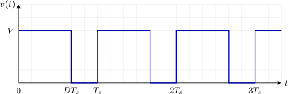
Before deriving the Fourier series, consider a simple periodic rectangular waveform. This waveform is one of the most important examples in power electronics because many switching waveforms can be approximated or directly represented by this form.
Let the waveform have:
- Amplitude \(V\),
- Switching period \(T_s\),
- Duty cycle \(D\), where \(0\le D\le1\).
The duty cycle is defined as the fraction of each switching period during which the waveform remains at \(V\):
Therefore, the ON-time is
and the remaining OFF-time is
We define the rectangular waveform over one period as follows:
and the waveform repeats every switching period:
Thus, the waveform has a value of \(V\) for a fraction \(D\) of every period and a value of zero for the remaining fraction \(1-D\).
Fundamental Period and Frequency
The fundamental period of the waveform is \( T_S \). Therefore, the fundamental frequency is \(f_s=1/T_s\), and the corresponding fundamental angular frequency is \(\omega_s=2\pi f_s=2\pi/T_s\).
The Fourier-series components occur at integer multiples of the fundamental frequency. Thus, the angular frequencies are \(\omega_s,2\omega_s,3\omega_s,\ldots\), or equivalently, the frequencies are \(f_s,2f_s,3f_s,\ldots\).
We can now derive the Fourier series from the general Fourier-series equations while keeping the duty cycle \(D\) arbitrary throughout the derivation.
Note that the rectangular waveform is periodic and discontinuous (piecewise-constant). During each switching period, the voltage remains at \(V\) for the ON-time \(DT_s\) and at zero for the remaining time \( (1-D)T_S \).
At \(t=DT_s\), the voltage changes instantaneously from \(V\) to zero. At the beginning of the next switching period, it returns to \(V\).
Thus, although the waveform is continuous between switching instants, it is discontinuous at the switching transitions.
Fourier Series Derivation
For the rectangular waveform, start from the general Fourier series:
with
The Fourier coefficients are
Since the waveform is \(V\) only during \(0\leq t<DT_s\) and zero for the remainder of the period, the coefficient calculations reduce to the ON interval.
DC Coefficient
Therefore,
Cosine Coefficient
Using \(\omega_s=2\pi/T_s\),
Sine Coefficient
Using \(\omega_s=2\pi/T_s\),
Substituting \(a_0\), \(a_n\), and \(b_n\) into the Fourier-series expression gives
The magnitude-phase form
where
Substituting \(a_n\) and \(b_n\),
Factor out \(V/(n\pi)\):
Expand the square:
Using \(\sin^2\theta+\cos^2\theta=1\),
Using the identity \(1-\cos(2x)=2\sin^2x\),
Therefore,
The absolute value is required because a magnitude is always non-negative.
The phase angle is
so
An equivalent and more compact phase expression can be obtained from the harmonic term itself:
Using the identities \(\sin(2x)=2\sin x\cos x\) and \(1-\cos(2x)=2\sin^2x\),
Using \(\cos(A-B)=\cos A\cos B+\sin A\sin B\),
Therefore, a compact magnitude-phase representation is
Special Case D=0.5
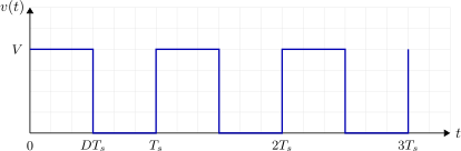
For a 50% duty cycle as shown in Figure 2, substitute \(D=0.5\) directly into the general Fourier-series result.
The DC component becomes
For the cosine coefficient,
For the sine coefficient,
Since \(\cos(n\pi)=(-1)^n\),
Therefore,
Thus, the Fourier series becomes
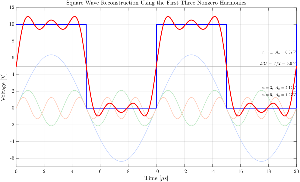
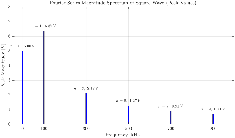
So, for \(D=0.5\), the waveform contains a DC component of \(V/2\) and only odd harmonics.
Special Case D=0.5 in Magnitude-Phase Form
For \(D=0.5\), the general harmonic magnitude
For even \(n\),
So all even harmonics vanish.
For odd \(n=1,3,5,\ldots\),
therefore
and
For the 50% duty-cycle waveform, the non-zero harmonics can be written with a phase of \(90^\circ\) in cosine form:
Equivalently,
This is the magnitude-phase form of the 50% duty-cycle rectangular waveform.